Strip Plot Analysis with Agri Analyze: From Basics to Solved Examples
The blog contains basics of strip plot design, randomization, ANOVA model, all the formulas and solved example along with demonstration in Agri Analyze. (Reading time 15 min.)
The Strip Plot Design (SPD) is particularly suitable for two-factor experiments where higher precision is needed for measuring the interaction effect between the factors compared to measuring the main effects of either factor individually. This design is also ideal when both sets of treatments require large plots. For instance, in experiments involving spacing and ploughing treatments, cultural convenience necessitates larger plots. Ploughing strips can be arranged in one direction, and spacing strips can be laid out perpendicular to the ploughing strips. This arrangement is achieved using:
- Vertical strip plot for the first factor (the vertical factor)
- Horizontal strip plot for the second factor (the horizontal factor)
- Interaction plot for the interaction between the two factors.
The vertical and horizontal strip plots are always perpendicular to each other. However, their sizes are unrelated, unlike the main plot and subplot in the split plot design. The interaction plot is the smallest. In a strip plot design, the precision of the main effects of both factors is sacrificed to improve the precision of the interaction effect.
Randomization and Layout Planning for Strip Plot
Design
Step
1: Assign horizontal plots by dividing the
experimental area into r blocks, then dividing each block into horizontal
strips. Follow the randomization procedure used in RBD, and randomly assign the
levels of the first factor to the horizontal strips within each of the r
blocks, separately and independently.
Step
2: Assign vertical plots by dividing each
block into b vertical strips. Follow the randomization procedure used in RBD
with b treatments and r replications, and randomly assign the b levels to the
vertical strips within each block, separately and independently.
Layout Example:
A sample layout of strip-plot design with six varieties (V1, V2, V3, V4, V5 and V6) as a horizontal factor and three nitrogen rates (N1, N2 and N3) as a vertical factor in three replications.

Example
of Strip Plot Design
In the previous chapter, this dataset
was used for a split-plot design and now the same dataset will be used to
illustrate a strip plot design.
A strip plot
design was used to investigate the effects of irrigation levels (Horizontal
factor) and fertilizer types (Vertical factor) on the yield of a particular
crop. The experiment was conducted over four replicates (R1, R2, R3, R4).
Factors:
Horizontal Factor (A - Irrigation
Levels):
A1: Low Irrigation
A2: Medium Irrigation
A3: High Irrigation
Vertical Factor (B - Fertilizer
Types):
B1: Organic Fertilizer
B2: Inorganic Fertilizer
B3: Mixed Fertilizer
|
Treatments |
R1 |
R2 |
R3 |
R4 |
|
A1B1 |
386 |
396 |
298 |
387 |
|
A1B2 |
496 |
549 |
469 |
513 |
|
A1B3 |
476 |
492 |
436 |
476 |
|
A2B1 |
376 |
406 |
280 |
347 |
|
A2B2 |
480 |
540 |
436 |
500 |
|
A2B3 |
455 |
512 |
398 |
468 |
|
A3B1 |
355 |
388 |
201 |
337 |
|
A3B2 |
446 |
533 |
413 |
482 |
|
A3B3 |
433 |
482 |
334 |
435 |
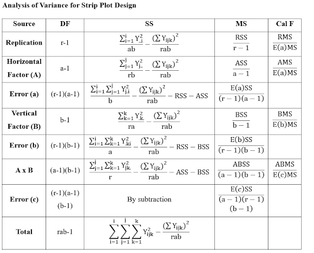
Final ANOVA Table for Crop Yield
Analysis Using Strip Plot Design with Irrigation and Fertilizer Treatments:
|
|
TABLE F |
|||||
|
SV |
DF |
SS |
MS |
CAL F |
5% |
1% |
|
Replication |
3 |
61636.97 |
20545.66 |
28.12 |
3.49 |
10.80 |
|
Horizontal plot (A) |
2 |
12391.17 |
6195.58 |
8.48 |
5.14 |
10.92 |
|
Error (A) |
6 |
4382.61 |
730.44 |
|
|
|
|
Vertical Plot (B) |
2 |
128866.67 |
64433.33 |
81.35 |
5.14 |
10.92 |
|
Error (B) |
6 |
4752.44 |
792.07 |
|
|
|
|
A X B |
4 |
304.17 |
76.04 |
0.62 |
3.26 |
5.41 |
|
Error (C) |
12 |
1462.72 |
121.89 |
|
|
|
|
Total |
35 |
213796.75 |
|
|
|
|
Calculation of degrees of freedom:
Replication DF: r-1 = 4-1=3
Main plot (A): a-1=3-1=2
Error (A): (r-1)*(a-1)=3*2=6
Main plot (B): b-1=3-1=2
Error (B): (r-1)*(b-1)=3*2=6
A x B: (a-1)*(b-1)=2*2=4
Error (C): (r-1)*(a-1)*(b-1)=3*2*2=12
Total: rab-1=4*3*3-1=35
Calculation of MS:
Replication:
61636.97/3=20545.66
Main
plot (A): 12391.17/2=6195.58
Error
(A): 4382.61/6=730.44
Main
plot (B): 128866.67/2=64433.33
Error
(B): 4752.44/6=792.07.
A
x B: 304.17/4=76.04
Error
(C): 1462.72/12=121.89
Conclusion:
·
The calculated F-value (28.12) is much greater than the critical
F-values at both 5% (3.49) and 1% (10.80) significance levels. Therefore,
there is strong evidence to suggest that there are significant differences
between the replicates.
·
The calculated F-value (8.48) for horizontal factor exceeds the
critical F-value 5% (5.14) significance levels. This indicates that there are significant
differences among the irrigation level.
·
The calculated F-value (81.35) for vertical factor exceeds the critical
F-value at 1% (10.92) significance level. This indicates that there is highly
significant variation among level of fertilizer.
·
The calculated F-value (0.62) for interaction between main factor and
sub factor (A x B) which is less than critical F-value at 5% (2.93)
significance level. This indicate that there is non-significant interaction
between irrigation and fertilizer.
·
For the irrigation, highest yield was observed for A1 and A2 were found
statistically at par with it based on critical difference.
·
For the fertilizer, highest yield was observed for B2 and none of the
level of fertilizer at par with it based on critical difference.
Steps to perform analysis of split plot design in
Agri Analyze
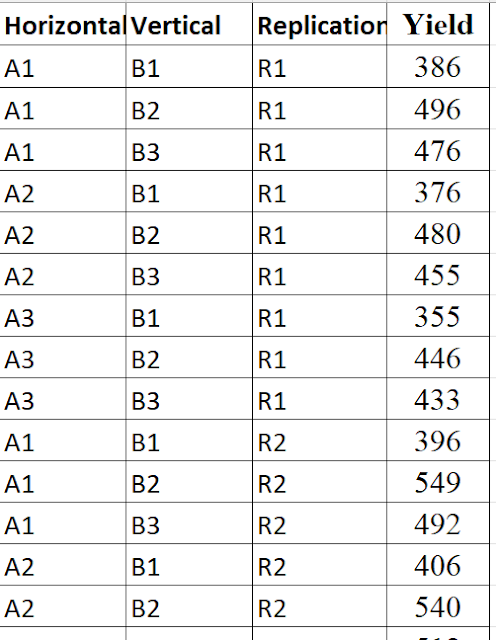
Step 1: To create a CSV file with columns for replication,
Horizontal factor (A), vertical factor (B) and Yield. Link of the dataset
Step 2: Go with Agri Analyze site https://agrianalyze.com/Default.aspx
Step 3: Click on ANALYTICAL TOOL
Step 4: Click on DESIGN OF EXPERIMENT
Step 5: Click on STRIP PLOT DESIGN ANALYSIS
Step6: Select CSV file
Step 7: Select Replication, Horizontal factor (A), Vertical factor (B) and Dependent variable (Yield)
Step 8: Select a test for multiple comparisons, such as Least Significant Difference (LSD) test or Tuckey's test or Duncan's New Multiple Range Test (DNMRT test) for grouping of treatment means.
Step 10: After submit
download analysis report.
Output Result
REFERENCES
Gomez, K. A., & Gomez, A. A. (1984). Statistical Procedures for Agricultural Research. John wiley & sons. 108-120.
This blog is written by:
Content Writer
Agri Analyze


Comments