Variability analysis in R - I: Genetic parameters
Step-I Arrangement of data in Excel file
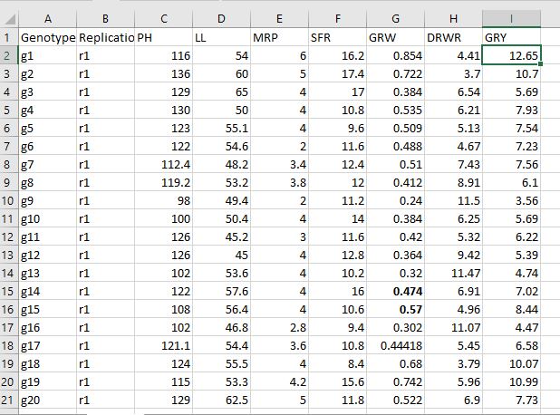
The data consist of 28 genotypes, 2 replication and 7 traits. First arrange genotypes followed by replication and than seven traits. The file is named vardata. You can download the excel file. Have a look at snip of data.
Step-II Import the excel data file in RStudio
On the upper right quadrant in RStudio there is tab of import dataset. Click on it and choose From Excel option. Browse for the excel file and click on import.

After successful import one can see the dataset in Global Environment by the name vardata
Step-III Import the variability package from CRAN
For our analysis we need a package named variability. Follow the below mentioned steps to install the package:
Click on Package
Click on install
Ensure "Repository (CRAN)" is selected in Install from option
Type name of package i.e. variability
Click on install
Make sure the system is connected to internet in order to download the package.
Step-IV R script
Lines in blue are script. Type these blue lines and press Ctrl+Enter run the lines.
Open a new script by clicking on New and than selecting R script or by pressing Ctrl+Shift+N.
Note: R is case sensitive
library(variability)
gen.var(vardata[3:9],vardata$Genotypes,vardata$Replication) gen.var is our function belonging to variability package
vardata[3:9] here square bracket are used for indexing. 3:9 means our data is located from column 3 to column 9 in "vardata" dataset
vardata$Genotypes is used to use genotypes as an input. R will look for a column named Genotypes in vardata dataset
vardata$Replication is used to use replication as an input. R will look for a column named Replication in vardata dataset
You can see the output in console. Select the output and copy paste it in word or text format as per your requirement.
Output
$PH
$PH[[1]]
Analysis of Variance Table

Response: data2
            Df Sum Sq Mean Sq F value    Pr(>F)
replication  1   25.1  25.112  0.4693 0.4991606
genotype    27 6285.1 232.782  4.3501 0.0001398 ***
Residuals   27 1444.8  53.512
---
Signif. codes:  0 ‘***’ 0.001 ‘**’ 0.01 ‘*’ 0.05 ‘.’ 0.1 ‘ ’ 1

$PH[[2]]
                                             A
Maximum                               139.0000
Minimum                                86.0000
Grand Mean                            116.3518
Standard Error of Mean (SEm)            5.1726
Critical Difference (CD) 5%            15.0095
Critical Difference (CD) 1%            20.2680
Environmental Variance                 53.5116
Genotypic Variance                     89.6352
Phenotypic Variance                   143.1468
Environmental Coefficient of Variance   6.2871
Genotypic Coefficient of Variance       8.1370
Phenotypic Coefficient of Variance     10.2830
Heritability (Broad Sense)              0.6262
Genetic Advance                        15.4332
Genetic Advance as percentage of mean  13.2643
$LL
$LL[[1]]
Analysis of Variance Table

Response: data2
            Df  Sum Sq Mean Sq F value    Pr(>F)
replication  1   32.47  32.467  2.2597 0.1443879
genotype    27 1680.93  62.257  4.3330 0.0001447 ***
Residuals   27  387.94  14.368
---
Signif. codes:  0 ‘***’ 0.001 ‘**’ 0.01 ‘*’ 0.05 ‘.’ 0.1 ‘ ’ 1

$LL[[2]]
                                            A
Maximum                               72.0000
Minimum                               40.5000
Grand Mean                            53.7971
Standard Error of Mean (SEm)           2.6803
Critical Difference (CD) 5%            7.7775
Critical Difference (CD) 1%           10.5023
Environmental Variance                14.3680
Genotypic Variance                    23.9443
Phenotypic Variance                   38.3123
Environmental Coefficient of Variance  7.0459
Genotypic Coefficient of Variance      9.0958
Phenotypic Coefficient of Variance    11.5056
Heritability (Broad Sense)             0.6250
Genetic Advance                        7.9689
Genetic Advance as percentage of mean 14.8129
.... analysis of another 5 traits (trimmed to save space)
How analysis by this package has edge over other tools?
$SFR
$SFR[[1]]
Analysis of Variance Table

Response: data2
            Df Sum Sq Mean Sq F value Pr(>F)
replication  1   1.26  1.2600  0.1664 0.6866
genotype    27 158.11  5.8561  0.7732 0.7458
Residuals   27 204.50  7.5741

$SFR[[2]]
                                      A
Maximum                               17.8
Minimum                               8.2
Grand Mean                            12.8714
Standard Error of Mean (SEm)          1.946
Critical Difference (CD) 5%           5.6469 NS
Critical Difference (CD) 1%           7.6252 NS
Environmental Variance                7.5741
Genotypic Variance                    Note: GV is negative -0.859
Phenotypic Variance                   6.7151
Environmental Coefficient of Variance 21.3815
Genotypic Coefficient of Variance     Note: GV is negative,GCV calculated by using
absolute GV 7.2006
Phenotypic Coefficient of Variance 20.1326
Heritability (Broad Sense) -0.1279
Genetic Advance -0.6829
Genetic Advance as percentage of mean -5.3055 For the SFR trait, genotype component in RBD analysis is non-significant which leads to genotype mean square less then residual mean square making genotypic variance negative. We should remove this traits from variability study.
The currently available packages and online analysis website misleads researchers by taking absolute value of genetypic variance. By carrying out analysis with this package, the researchers will get note when the genotypic variance is negative.
Suggestions, Comments and Quires are welcomed
Happy Learning!
If you prefer watching content over reading it, tune to YouTube video
If you are using the variability R package in research work you can cite it as:


Comments
Regards
RAAJ