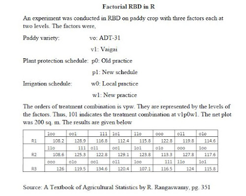
Factorial Randomized Block Design along with LSD test in R

The post explains how to get FRBD ANOVA, Interpretation of ANOVA, R-square, Normality assumption testing, Least significant difference (LSD) test using doebioresearch package in RStudio (Reading time 12 min.)

Click here for data and Click here for R-script

Factors: 3  Levels: 2 Replication:3  and dependent variables Yield & Plant Height

Click on the link given in top to get the data arranged in excel. Get a closer look on data arrangement.

R-script

#You can upload the data by clicking on import data set-> From Excel -> Browse -> Select your file-> #Import

#This line will load doebioresearch package
library(doebioresearch)

#This line will store the analysis obtained from function frbd3fact in output variable

output<-frbd3fact(FRBD[5:6],FRBD$R,FRBD$V,FRBD$P,FRBD$W,1)
output

#This line will use sink function to store the output variable present in global environment in output.doc

sink("output.doc")
print(output)
sink()

Output and interpretation

Click here to get entire result

Analysis of Variance Table

Response: dependent.var

                     Df Sum Sq Mean Sq F value   Pr(>F)  

replicationvector     2  61.06   30.53  1.4112 0.276494  

fact.A                1 320.47  320.47 14.8123 0.001772 **

fact.B                1  56.12   56.12  2.5939 0.129584  

fact.C                1 154.53  154.53  7.1426 0.018208 *

fact.A:fact.B         1 272.70  272.70 12.6043 0.003199 **

fact.A:fact.C         1   0.22    0.22  0.0102 0.921034  

fact.B:fact.C         1   3.60    3.60  0.1666 0.689355  

fact.A:fact.B:fact.C  1   3.01    3.01  0.1391 0.714722  

Residuals            14 302.90   21.64                   

---

Signif. codes:  0 ‘***’ 0.001 ‘**’ 0.01 ‘*’ 0.05 ‘.’ 0.1 ‘ ’ 1 

The ANOVA shows Fact.A (Paddy variety), Fact.C (Irrigation schedule) and Fact.A*Fact.B (Paddy variety*Plant protection schedule) were significant. We will ignore the the LSD results of rest of the combination of the factors and interaction.

[1] "R Square 0.742"

0.742 i.e. 74.20% of variation present in the dependent variable is explained by the model.

[1] "SEm of A: 1.343 , SEd of A: 1.899 , SEm of B: 1.343 , SEd of B 1.899 , SEm of C: 1.343 , SEd of C: 1.899 , SEm of AB: 1.899 , SEd of AB: 2.685 , SEm of AC: 1.899 , SEd of AC: 2.685 , SEm of BC: 1.899 , SEd of BC: 2.685 , SEm of ABC: 2.685 , SEd of ABC: 3.798"

Shapiro-Wilk normality test

data:  model$residuals

W = 0.98223, p-value = 0.9332

[1] "Normality assumption is not violated"

[1] "The means of one or more levels of factor A are not same, so go for multiple comparison test"

   MSerror Df     Mean       CV  t.value      LSD

  21.63548 14 119.6458 3.887636 2.144787 4.072787

   dependent.var groups

v0      123.3000      a

v1      115.9917      b

Paddy variety vo (ADT-31) gives highest yield which is significantly different from v1 (Vaghai)

[1] "The means of one or more levels of factor C are not same, so go for multiple comparison test"

   MSerror Df     Mean       CV  t.value      LSD

  21.63548 14 119.6458 3.887636 2.144787 4.072787

   dependent.var groups

w1      122.1833      a

w0      117.1083      b

The irrigation schedule new practice gives highest yield which is significantly different from the local practice

[1] "The means of levels of interaction between A and B factors are not same, so go for multiple comparison test"

   MSerror Df     Mean       CV  t.value      LSD

  21.63548 14 119.6458 3.887636 2.144787 5.759791

      dependent.var groups

v0:p0      128.2000      a

v0:p1      118.4000      b

v1:p1      117.8333      b

v1:p0      114.1500      b

The combination v0p0 (ADT-31*old practice) has highest yield which is significantly different from the rest of three combinations.

If you are using "doebioresearch" for analysis. You can cite it as:

Popat, R and Banakara, K. (2020). doebioresearch: Analysis of Design of Experiments for Biological Research. R package version 0.1.0

To learn more about Agricultural Statistics follow my YouTube channel

Happy Learning!

Bored of reading? Tune to video!

Reference:

Rangaswamy, R. (2010). A textbook of Agricultural Statistics (2ndedn). New Age International Publishers, New Delhi.

 

Topics you might be interested in:

Split plot analysis in R