Pearson Correlation along with p values and fancy graphs in R

The blog explains correlation analysis in R (Reading time 10 min.)
For data click here and for R-script click here

The Pearson correlation coefficient is a measure of the strength of a linear association between two variables and is denoted by r. The value of r ranges between -1 to +1. Let's see how to calculate correlation, the test of significance and fancy graphics to explain the relationship between variables in R.

Step-I: Import the data

In the II quadrant click on import data and select "For Excel".

After that new dialogue box appears, click on "browse" and select your file and click on "import".

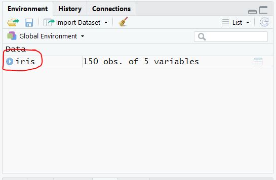
After doing this step the "iris" data gets imported in the system and can be seen in Global Environment.

Step-II: Load the script which you had downloaded.

Let's understand the script step by step.

Calculating the correlation and p values

#Gives structure of the data
str(iris)

tibble [150 x 5] (S3: tbl_df/tbl/data.frame)
 $ Sepal.Length: num [1:150] 5.1 4.9 4.7 4.6 5 5.4 4.6 5 4.4 4.9 ...
 $ Sepal.Width : num [1:150] 3.5 3 3.2 3.1 3.6 3.9 3.4 3.4 2.9 3.1 ...
 $ Petal.Length: num [1:150] 1.4 1.4 1.3 1.5 1.4 1.7 1.4 1.5 1.4 1.5 ...
 $ Petal.Width : num [1:150] 0.2 0.2 0.2 0.2 0.2 0.4 0.3 0.2 0.2 0.1 ...
 $ Species     : chr [1:150] "setosa" "setosa" "setosa" "setosa" ...

We can see from output that the first 4 variables are numeric (num) and the last one is character (chr).

The code below will install the package named "psych". Make sure that system is connected to the internet.

install.packages("psych")

Note: This line is run for once only. This will install "psych" in system. Next time when we need psych we just load that package.

library("psych")

This line will load the package psych

b<- corr.test(iris[1:4])
The corr.test function saves correlation (r), t values of t-test (t), p-values (p) and standard error (se) in the variable named "b".

"<-" is used to assign the output to variable b

iris[1:4] is used because we want the first four variables as the fifth variable is a character in nature.

b$r

gives a correlation matrix. "$" is used to extract components stored in "b"

           Sepal.Length Sepal.Width Petal.Length Petal.Width
Sepal.Length    1.0000000  -0.1175698    0.8717538   0.8179411
Sepal.Width    -0.1175698   1.0000000   -0.4284401  -0.3661259
Petal.Length    0.8717538  -0.4284401    1.0000000   0.9628654
Petal.Width     0.8179411  -0.3661259    0.9628654   1.0000000

b$t

gives t statistic value

             Sepal.Length Sepal.Width Petal.Length Petal.Width
Sepal.Length          Inf   -1.440287    21.646019   17.296454
Sepal.Width     -1.440287         Inf    -5.768449   -4.786461
Petal.Length    21.646019   -5.768449          Inf   43.387237
Petal.Width     17.296454   -4.786461    43.387237         Inf

b$p
gives p-value

            Sepal.Length  Sepal.Width Petal.Length  Petal.Width
Sepal.Length 0.000000e+00 1.518983e-01 5.193337e-47 9.301992e-37
Sepal.Width  1.518983e-01 0.000000e+00 1.353994e-07 8.146457e-06
Petal.Length 1.038667e-47 4.513314e-08 0.000000e+00 2.805002e-85
Petal.Width  2.325498e-37 4.073229e-06 4.675004e-86 0.000000e+00

b$se

gives standard error

            Sepal.Length Sepal.Width Petal.Length Petal.Width
Sepal.Length   0.00000000  0.08162941   0.04027317  0.04728953
Sepal.Width    0.08162941  0.00000000   0.07427301  0.07649200
Petal.Length   0.04027317  0.07427301   0.00000000  0.02219237
Petal.Width    0.04728953  0.07649200   0.02219237  0.00000000

sink("correlation.doc")
print(b)
sink()

The sink function will store the "print(b)" into a document file named "correlation" (You can change the name as per your wish). The document gets stored working directory which can be obtained by using getwd().

Visualization of correlation

pairs.panels(iris[,-5],pch = 21,stars = T)

iris[,-5] is used as we don't want the fifth variable which is a character in nature

pch=21 will give circles in the scatters plot (You can try different numbers)

stars=T will five stars in the figure to indicate significant or non-significant

One can save the plot in image or pdf form by using the Export option of plot section

The upper triangle of the matrix shows correlation values, diagonal shows the distribution of the variable and the lower triangle of the matrix shows the scatter distribution of variables.

install.packages("PerformanceAnalytics")
The above code will install "PerformanceAnalytics". (Internet on!)

Run the code one time only.

require("PerformanceAnalytics")

This function is similar to library(). This will load the package.

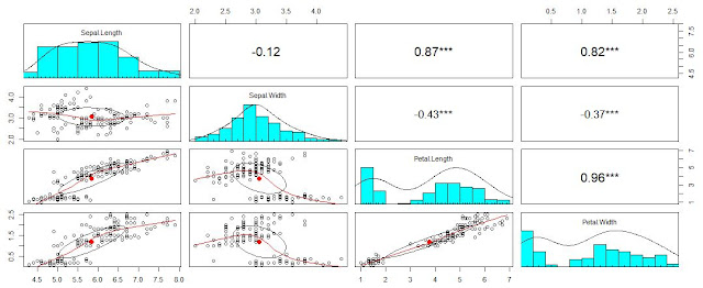
chart.Correlation(iris[1:4], histogram = TRUE, pch = 100)

In comparison to pervios function here the values of correlation are proportional to their size. The larger the value the greater the size.

detach("package:psych", unload=TRUE)
This will unload the package "psych"

detach("package:PerformanceAnalytics", unload=TRUE)
This will unload the package "PerformanceAnalytics"

Bored of reading? Tune to video!